Autoorbit Mechanics

In my Drone Simulation Project I have thought about orbits in eve quite a lot. The general behaviour of objects in eve online is well understood. For example Dr. Santorine has generated some really cool explanations in the past. It is pretty much possible to calculate exactly how yourr ship will move with a given set of input commands.

Dr. Santorine also proposed a model that calculates the autoorbit speed at any given distance for any given ship. Sadly these values don’t always line up exactly with what can be observed in game. Specifically at really tight orbits there seems to be difficulty, the model also has a sharp corner in it’s function which couldn’t be observed in game.

Orbit Mechanics

You are probably familiar with the Orbit button in Eve. You set it to Orbit at a certain distance (say 500 m) and then your actual trajectory ends up a little further out (800 m or so) all the while, you constantly accelerating and thus not quite reaching top speed. Dr. Santoine assumed that this trajectory a little further out is a circle. Given that the eve velocity formulas are continuous, that makes a lot of sense. Here are the formulas that we are talking about:

• \( \vec{v}_{max} \qquad \) Denotes the vector where your ship is planning to go e.g.
  • where you double clicked,
  • the direct line to someone that you are approaching
• \( |\vec{v}_{max}| \qquad \) Is capped to your ships maximum speed.
• \( \vec{v}_0 \qquad \) Is the current trajectory of your ship
• \( I \qquad \) Denotes your ships intertial modifier
• \( M \qquad \) Denotes your ships mass
• \( t \qquad \) is the time passed

\( \vec{a}(t) = (\vec{v}_{ max} – \vec{v}_ 0) \cdot \frac{10^6 }{IM} \cdot e^{-t \cdot \frac{10^6 }{IM}} \qquad (1) \)

\( \vec{v} (t) = (\vec{v}_{ max} – \vec{v}_ 0) \cdot (1−e^{-t \cdot \frac{10^6 }{IM}}) + \vec{v}_ 0 \qquad (2) \)

\( \vec{d} (t) = (\vec{v}_{ max} – \vec{v}_ 0) \cdot (\frac{IM}{10^6 } \cdot (e^{-t \cdot \frac{10^6 }{IM}} -1) + 1 ) + \vec{v}_ 0 \qquad (3) \)

But there is in fact a thing hidden in here that could be discrete. The \( \vec{v}_{ max} \) Vector! If you ever manual piloted, then you probably realized that doubleclicking more often than once a second doesn’t really change anything, as the vector only changes once per tick. Dr. Santoine assumed that this is merely a limitation of how we can give inputs into Eve, but doesn’t actually affect the calculations within Eve. So if you click autoorbit, then your ship will continuously change this \( (\vec{v}_{ max} \) vector to make the best possible orbit.

I on the other hand propose that this update rate limit for the target vector always applies, even when autoorbiting. This based of the following Observation: Take any drone, let it shoot something and observe it’s trajectory. You can clearly see it being some rounded down polygon and not a precise circle. You can also see the effect when you look at your ship’s speed while orbiting, but due to the much higher mass the effect is a lot weaker.

With all this, I don’t think eve’s orbits are circles, they are something that is almost a circle, stitched together out of parts that follow the equations of motion above.

• The distance to the center stays constant
• The speed at a tick stays constant (It can do things in between ticks, but we don’t care about that)

Formula Derivation (Math Warning)

Setting \( t = 1 \) we can get two vector relations. The first one gives us the trajectory

\( \vec{v}_1 = (\vec{v}_{ max} – \vec{v}_ 0) \cdot (1−e^{- \frac{10^6 }{IM}}) + \vec{v}_ 0 \qquad (4) \)

While the second one gives us the distance traveled during that one tick

\( \vec{d}_{01} = (\vec{v}_{ max} – \vec{v}_ 0) \cdot (\frac{IM}{10^6 } \cdot (e^{- \frac{10^6 }{IM}} -1) + 1 ) + \vec{v}_ 0 \qquad (5) \)

I use \( \vec{v}_1 \) and \( \vec{d}_{01} \) instead of something like \( \vec{v}(1) \) to make their discrete nature at the tick clear. I am unsure what exactly eve calculates in between ticks (if anything). But for use there will only be these values for velocity at each tick, and distances between the two ticks.

We further get the velocity constraint that I had formulated in text earlier.

\( v_{actual} = | \vec{v}_0 | = | \vec{v}_1 | \qquad (6) \)

I will substitute \( v_{actual} \) whenever possible for now on to have as few variables as possible. You can think of this variable as the speed you can actually see your ship mooving at independent of the direction.

We can now start solving this problem. Combining the Equations 4 and 5 we can get rid of \( \vec{v}_{ max} \)

\( \vec{d}_{01} = (\vec{v}_1 – \vec{v}_ 0) \cdot \frac{\frac{IM}{10^6 } \cdot (e^{- \frac{10^6 }{IM}} -1) + 1 }{ 1−e^{- \frac{10^6 }{IM}} } + \vec{v}_ 0 \qquad (7) \)

This is a rather ugly formula, but looking at it in a geometrical sense we can make it useful anyway. The first term with \( \vec{v}_1 – \vec{v}_ 0 \) is perpendicular to \( \vec{d}_{01} \). So instead of dealing with this complicated term, we can just simply look at it in a geometrical sense to get a much simpler relation for the length of \( d_01 \). Here is a quick sketch:

The angle \( \alpha \) denotes the amount that we have rotated in that single tick around the center. Because the geometry is an isosceles triangle we can figure out the angele between \( \vec{v}_{0} \) and \( \vec{d}_{01} \) is \( \alpha/2 \) . And then because we know that the projection of \( \vec{v}_{0} \) is exactly as long as \( \vec{d}_{01} \) (the complicated term is perpendicular to \( \vec{d}_{01} \)) we can simply use trigonometry to figure out \( \vec{d}_{01} \)‘s length. So we get:

\( |\vec{d}_{01}| = | \vec{v}_0 | \cdot cos(\alpha / 2) = v_{actual} \cdot cos(\alpha / 2) \qquad (8) \)

We can find another simple geometric relation in the triangle using \( r_{actual} \) which is the distance our orbit settles at

\( |\vec{d}_{01}|^2 = 2 r_{actual}^2 (1 – cos(\alpha)) \qquad (9) \)

Combining the Equations 8 and 9 and solving for \( cos(\alpha) \) we get

\( 2 r_{actual}^2 (1 – cos(\alpha)) = v_{actual}^2 cos(\alpha / 2)^2 \)

\( cos(\alpha) = \frac{4r_{actual}^2 + v_{actual}^2}{ 4r_{actual}^2 – v_{actual}^2 } \qquad (10) \)

Now we can go back to Equation 1 and write it without any vector calculations, just the law of cosines and the length of each vector.

\( |\vec{v}_{max}|^2 \cdot (1−e^{- \frac{10^6 }{IM}}) = |\vec{v}_1|^2 + |\vec{v}_0|^2 ( e^{- \frac{10^6 }{IM}}) ^2 – 2 |\vec{v}_0|^2 e^{- \frac{10^6 }{IM}} cos(\alpha) \)

\( |\vec{v}_{max}|^2 \cdot (1−e^{- \frac{10^6 }{IM}}) = v_{actual} ^2 \left(1 + ( e^{- \frac{10^6 }{IM}}) ^2 – 2 e^{- \frac{10^6 }{IM}} cos(\alpha)\right) \)

Now we substitute \( cos(\alpha) \) with Equation 10:

\( |\vec{v}_{max}|^2 \cdot (1−e^{- \frac{10^6 }{IM}}) = v_{actual} ^2 \left(1 + ( e^{- \frac{10^6 }{IM}}) ^2 – 2 e^{- \frac{10^6 }{IM}} \frac{4r_{actual}^2 + v_{actual}^2}{ 4r_{actual}^2 – v_{actual}^2 } \right) \qquad (11) \)

And finally we solve for \( v_{actual} \)

\( v_{actual} = \sqrt{\frac{-k^2\left(4r_{actual}^2+ |\vec{v}_{max}| ^2\right) + \sqrt{k^4\left(4r_{actual}^2 + |\vec{v}_{max}| ^2\right) + 16 (k-2)^2 |\vec{v}_{max}| ^2k^2r_{actual}^2}}{2(k-2)^2}}\) with \( k = 1−e^{- \frac{10^6 }{IM}} \)

This is actually only one of the 4 possible solutions, but it is the one that we are interested in. A more friendly to read version of the formula would be something like this

\( k = 1−e^{- \frac{10^6 }{IM}} \)

\( a = (k-2)^2 \)

\( b = k^2(4r_{actual}^2 + |\vec{v}_{max}| ^2) \)

\( c = -4 |\vec{v}_{max}| ^2 r_{actual}^2 k^2 \)

\( v_{actual} = \sqrt{\frac{-b + \sqrt{b^2 – 4ac}}{2a}}\)

I am not sure if this is actually the fastest way to get to the result, or if there is things that I did that are totally not needed. With the same constraints it should also be possible to figure out the relationship between the selected orbit radius and the actual orbit radius. I haven’t done this calculation (yet).

I was further able to figure out the selected radius based of the actual radius and velocity. So far I haven’t reversed this formula, but it is definitely (and useful) possible as well.

\( r_{selected} = r_{actual} \cdot \left( \frac{k^2w^2+ v_{actual} ^2 ((1-k)^2 -1)}{2kwv_{actual}} \right) \)

Testing

I ran a number of tests to see if this formula actually works as intended. The tests can be found here.

Out of the 49 experiments I did:

• 44 resulted in an error of less than 0.5%
• 2 had an error between 0,5% and 2%
• 3 could not be used as the in game distance measurement for distances >10km is rounded to the kilometer, and as such does not have the necessary accuracy to make any good conclusion.

Graphs

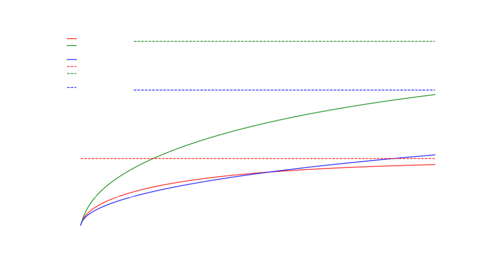
Taking the formula as valid, here is how the orbit speed should look like based on the distance that the ship settles in for a few select cases.

Here are different kinds of Jaguars. You can clearly see that some of the cases saturate much faster than others. It would be really interesting to plot the graph for this one with the selected orbit distance as well, as there is definitely some cases very close to 0 that aren’t actually possible. It should be noted that this speed is always achieved at the tick. In between the ticks the speed might be slightly different.

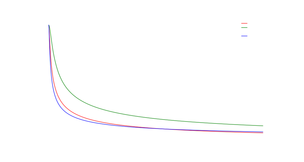
His is the same cases, but now plotting the angular velocity. It looks like orbiting with a prop mod that makes you faster generally gives you more angular velocity, which kinda makes sense. Again the values all the way on the left are not actually achieveable, as you always need to add something to your selected orbit.

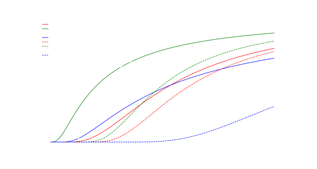
Here is the application of a gun with 200 Tracking and 1 DPS. The dashed lines are the application without taking into effect the reduced orbiting speed, as it is currently used in pyfa.

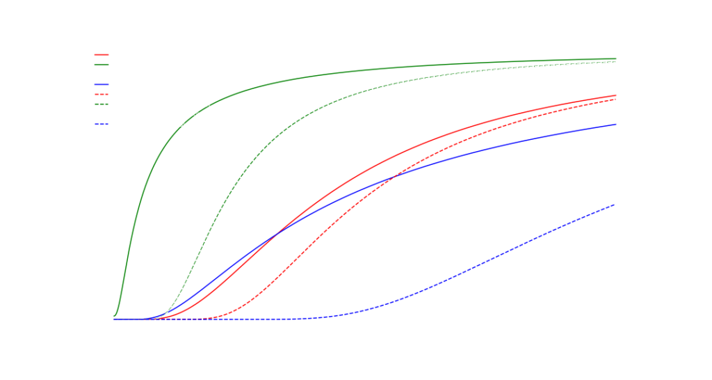
As the Jaguar is signature bonused this doesn’t translate well to other hulls. Because of that I decided to make another graph with the same thing, but for a Kikimora. I also changed the gun to only have 100 tracking in this one to adjust for the slower ship and bigger signature.

Further Ideas

I was mainly interested on what kind of effect this has on tracking performance, and as such have always started from \( r_{actual} \). There would definitely be some cool use from solving the same problem for \( r_{selected} \) at this point it is only a matter of algebraics – that I got enough of recently.

On behalf of graphing the tracking on different ships, the effects of limited acceleration seem to be mostly noticable in the sub 10 km range and with Microwarpdrives or Oversized Propmods. There is definitely some cases where current damage graphing techniques as used in pyfa produce significantly different results from what is observed in game, but there is also cases where the difference is rather small.

I further want to note that in my proposed model of autoorbits there is no fundamental difference to manual piloting. So orbiting a stationary target with manual orbiting or automatic orbiting will result in the same slowdown. The manual piloting obviously has other benefits like being able to choose the orbit plane and reacting to change in the targets movement more quickly.